Dimension reduction using python

Dimension Reduction
In Machine learning each feature or columns is called as dimension. Reducing the number of column or feature is called as a dimension reduction. Dimension reduction is important because it helps our model to predict more accurate output as it gets less confused.
Will perform the dimension reduction on this kaggle data set Churn_Modelling.csv
Methods of dimension reduction
- Correlation.
- Backward Elimination.
- PCA.
- Feature Importance.
1. Correlation
- Correlation is one of the methods used for dimension reduction.
- It is done to find out if there are any similarities between the two columns.
- If there is any correlation between two variable we drop one of them which in turn reduces the number of input variables to our model.
- Python to reduce the dimension using the correlation is shown below.
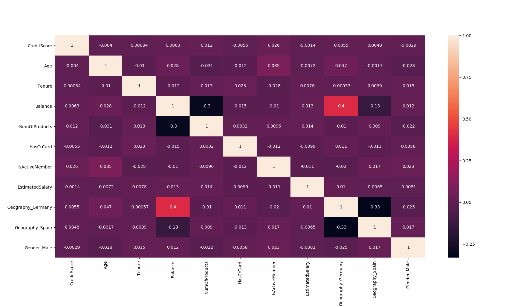
import seaborn as sns
corr = X.corr()
ax = sns.heatmap(corr, annot=True)
bottom, top = ax.get_ylim()
 |
|---|
| Correlation Heatmap. |
- In the above heatmap you see the correlation coefficient you can set threshold if it is above threshold value you can drop that column be it positive or negative.
2. Backward Elimination
- In backward elimination there few steps which are need to be followed.
- Firstly you have to select the significance value (p=0.05).
- If significance value of a particular column is above 0.05 we will drop that column.
- First you have to fit the with all the input features you have then check for the p values of the all the features. If features have p>0.05 then check for the feature which has highest p value compared to other features then drop that feature and fit again with remaining features.
- Repeat the above step till the p<0.05 for all the features.
- Code shown below
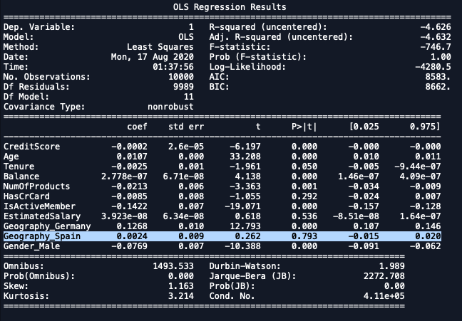
1st Iteration
import statsmodels.regression.linear_model as sm
x_formated = X.loc[:,['CreditScore', 'Age', 'Tenure', 'Balance',
'NumOfProducts','HasCrCard','IsActiveMember',
'EstimatedSalary', 'Geography_Germany',
'Geography_Spain', 'Gender_Male']]
ols = sm.OLS(endog = y, exog = x_formated).fit()
ols.summary()
 |
|---|
| Dropping Geography_Spain. |
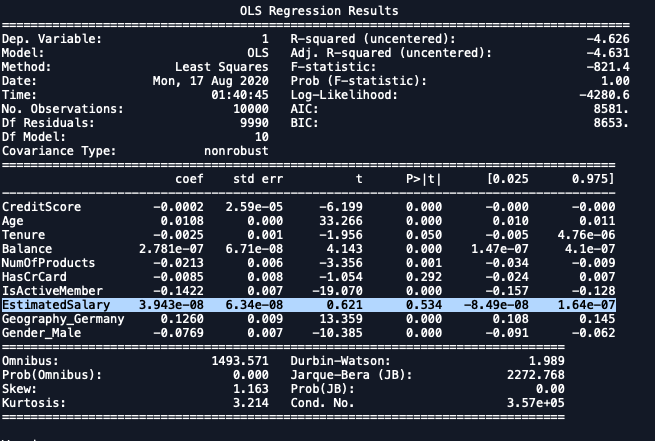
2nd Iteration
import statsmodels.regression.linear_model as sm
x_formated = X.loc[:,['CreditScore', 'Age', 'Tenure',
'Balance', 'NumOfProducts', 'HasCrCard',
'IsActiveMember', 'EstimatedSalary',
'Geography_Germany','Gender_Male']]
ols = sm.OLS(endog = y, exog = x_formated).fit()
ols.summary()
 |
|---|
| Dropping EstimatedSalary. |
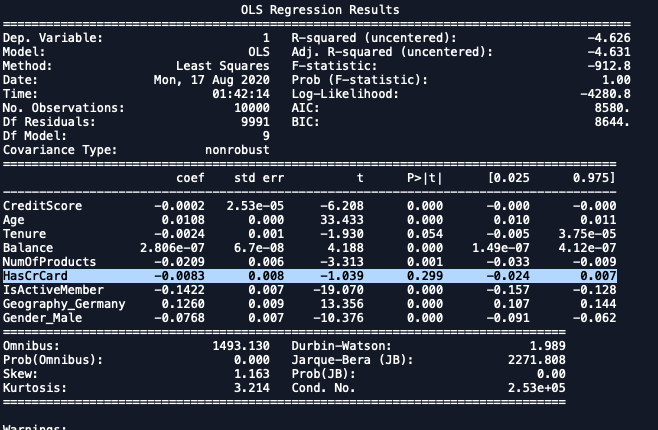
3rd Iteration
import statsmodels.regression.linear_model as sm
x_formated = X.loc[:,['CreditScore', 'Age', 'Tenure',
'Balance', 'NumOfProducts', 'HasCrCard',
'IsActiveMember', 'EstimatedSalary',
'Geography_Germany','Gender_Male']]
ols = sm.OLS(endog = y, exog = x_formated).fit()
ols.summary()
 |
|---|
| Dropping HasCrCard. |
4th Iteration
import statsmodels.regression.linear_model as sm
x_formated = X.loc[:,['CreditScore', 'Age', 'Tenure',
'Balance', 'NumOfProducts','IsActiveMember',
'Geography_Germany','Gender_Male']]
ols = sm.OLS(endog = y, exog = x_formated).fit()
ols.summary()
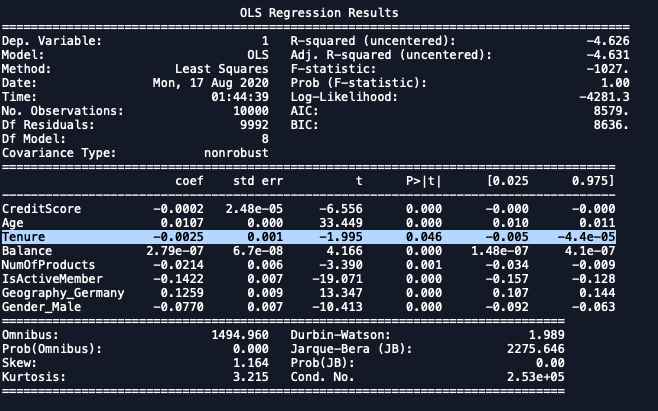 |
|---|
| No column has value p>0.05. |
3. Principal Component Analysis
- PCA is widely used for dimension reduction.
- It gives us the subset of the complete dataset.
- It preserves as much data present in the whole data set in small dimension.
- Code for the PCA is shown below.
from sklearn.decomposition import PCA
#n_components is number of columns you want merge the data
pca = PCA(n_components=2)
pca.fit(X)
print(pca.explained_variance_ratio_)
print(pca.singular_values_)
X_pca = pca.transform(X)
4. Feature Importance
- This method helps us to predict which feature contributes how much in predicting the output.
- It is done after the model is trained.
model.feature_importances_